How should a gambler with insider information bet?
In this article, you will learn a derivation of what is known as the Kelly criterion. The derivation I present here would be understood by an A-level maths student who has studied the S1 maths module and so is familiar with the concept of expected values. Knowledge of how to differentiate the function ![]() is needed (C3 maths). If you’ve not yet studied those, you are still encouraged to read through this and look up what you don’t understand in an A-level maths textbook. Questions and comments are also welcome.
is needed (C3 maths). If you’ve not yet studied those, you are still encouraged to read through this and look up what you don’t understand in an A-level maths textbook. Questions and comments are also welcome.
Through the Wire
It is the early 1900s, long before instantaneous live sports coverage. Gambling is very popular in the United States.
You are a corrupt telegraph operator, providing a ‘private wire’ service that transmits messages reporting horse racing results to anyone who can afford to pay you. You have an employee stationed at the local racetrack. The instant a horse crosses the finish line, the employee uses a hand mirror to flash the winner, in code, to another employee in a nearby building. This employee then telegraphs the results to your customers across the country.
Without your service it would take several minutes for someone to learn which horse has won. A bettor who knew the winner before a bookmaker could place bets on a horse that had already won. A bookmaker who knew the results before a better could refuse any bets on the horse that had already won, and of course, accept any bets on a horse that had already lost.
This is one example of inside information. You know the true odds of the horse winning, in this case certainty i.e. odds of 1, but you are allowed to place a bet at the bookmakers (less accurate) odds and thus profit. In this situation where the true odds are certainty, you would bet your entire bankroll.
‘I Keep Defying The Odds, You Know’
Suppose I have a biased coin, which when tossed has a probability of 51% of landing heads up and a probability of 49% of landing tails up. You have a bankroll of £100. You play a game where you can bet any amount (up to your entire bankroll) on the coin landing tails up. If it does you win the amount you bet plus your original stake, which adds to your bankroll. But if it does not, you lose your stake. You are allowed to play the game as many times as you like, unless your bankroll hits zero in which case you are ‘bankrupt’.
It can be proved mathematically that you will always end up bankrupt – in the long run. This will happen no matter how creative your system for deciding how to size your bets. We describe such situations by saying: the odds are not in your favour, and that there is a house edge. This in-built house edge allows casinos and bookmakers to profit in the long run, and customers to lose more than they win.
Now lets play the game again, but this time betting on heads. The probability of heads is 51%. You now have an edge, the odds are in your favour. It can proved that – in the long run – your bankroll will increase.
If you do have an edge, the question now is how do you size your bets? If you just bet your entire bankroll, there is a chance of going bankrupt. The other extreme is to bet zero, which would not change your bankroll at all. What could we define as an optimum amount to bet? What is the appropriate betting strategy?
 Enter John Kelly Jr
A scientist by the name of John Kelly Jr solved this problem by considering the optimum amount to bet to be that which maximises the expected rate of return of the bet. You will learn in S1 A-level maths that the term expected value or expectation value has a precise mathematical definition.
Suppose our starting bankroll, or wealth, is ![]() . Each time we place a bet, our wealth will be multiplied by a random variable
. Each time we place a bet, our wealth will be multiplied by a random variable ![]() . Our wealth after
. Our wealth after ![]() bets is
bets is
(1) ![]()
where ![]() are the
are the ![]() random outcomes of our bets.
random outcomes of our bets.
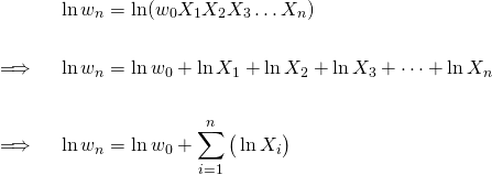
Taking natural logarithms of both sides of equation 1, we have
(2) 
If you have studied S1 A-level maths, you will know that we can write the expected value of the random variable ![]() as
as
(3) 
Substituting equation 3 into equation 2, gives
(4) 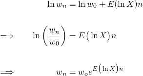
This equation gives our wealth after ![]() bets. Caution is needed here, because this equation only applies as
bets. Caution is needed here, because this equation only applies as ![]() (do you know why?).
(do you know why?).
We can now derive an expression for the average rate of return per bet.
Our average increase in net worth for each bet is ![]() . So we can write, using equation 4,
. So we can write, using equation 4,
(5) ![Rendered by QuickLaTeX.com \begin{equation*} \begin{aligned} w_{n+1} - w_n &= w_o e^{E(\ln X)(n+1)} - w_o e^{E(\ln X)n} \\ \\ &= w_o e^{E(\ln X)n}\big[e^{E(\ln X)} - 1\big] \\ \\ &= w_n \big[e^{E(\ln X)} - 1\big] \end{aligned} \end{equation*}](http://www.maxbenjamintutor.com/wp-content/ql-cache/quicklatex.com-23316525134e681a12db21b3adcc3ab2_l3.png)
Hence, the average rate of return per bet is
(6) ![]()
The Kelly Criterion
Suppose you have a simple bet where there is a probability ![]() of making a profit of
of making a profit of ![]() times what you bet, and otherwise you lose your bet. You are free to choose any fraction
times what you bet, and otherwise you lose your bet. You are free to choose any fraction ![]() of your bankroll as your stake for each bet. What amount should you bet?
of your bankroll as your stake for each bet. What amount should you bet?
John Kelly’s insight was that the optimal amount to bet is that which maximises the average rate of return. From this and our previous derivations, we can calculate the optimal value of ![]() (see if you can do this by yourself without reading further).
(see if you can do this by yourself without reading further).
We want to maximise the average rate of return per bet:
![]()
with respect to ![]() .
.
We can take a shortcut by noticing that this is equivalent to maximising ![]() .
.
From S1 A-level maths, the expected value of a random variable ![]() is
is
(7) ![]()
Hence, we can write the expected value of ![]() in terms of
in terms of ![]() ,
,
(8) ![]()
Differentiating this with respect to ![]() (see C3 A-level maths for differentiating
(see C3 A-level maths for differentiating ![]() ), we have
), we have
(9) 
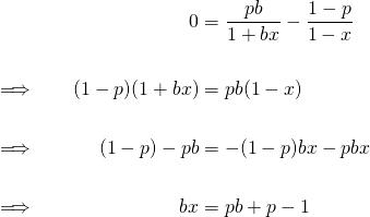
We can now find the value of ![]() which gives the maximum value of
which gives the maximum value of ![]() by setting the derivative, equation 9, equal to zero. Hence,
by setting the derivative, equation 9, equal to zero. Hence,
(10) ![]()
This important result is known as the Kelly criterion. It gives the optimal value of ![]() , the fraction of our bankroll that we should bet in order to maximise the average rate of return per bet, given the probability
, the fraction of our bankroll that we should bet in order to maximise the average rate of return per bet, given the probability ![]() of winning the bet and the profit multiple
of winning the bet and the profit multiple ![]() .
.
 It should be noted that the Kelly criterion says what to do to maximise the average rate of return in the long run. That is to say, the more and more bets you make the better off you will be compared to anyone else who uses a different staking system. In the short term, there can be quite a bit of fluctuation in your bankroll.
As a final point, it also says to only gamble if you have an edge – and there are no casino games like that.
Further exercises
- Prove that when the odds are not in your favour, i.e. negative edge, you will go bankrupt in the long run. You must write a correct mathematical proof and use correct mathematical notation.
- Research the Martingale betting system, and prove mathematically that unless there is an edge it leads to bankruptcy in the long run. Pick two more betting systems and prove the same thing.
- Write a 2,000 word report about a situation in a casino which would give you an edge. Two examples you could write about are card-counting in Blackjack and edge-sorting in Baccarat. Include relevent maths.
- So far we have looked at the idealised case where the true odds of winning the bet are known to you. Describe some scenarios where the true odds change but are not known fully, possibly a piece of insider information regarding a horse running in a race – you can pick as many examples as you wish. How would you deal with these situations quantitatively? Try and think like a physicist when investigating this.
- The simple derivation here considered a simple bet where you have an edge. Think about other situations, such as a horse race where you have an edge on several horses. How would the Kelly criterion be modified for this? Pick two more situations, describe them and explain how the Kelly criterion would apply.
Further Reading
- The Kelly Capital Growth Investment Criterion, Leonard C. Maclean, Edward O. Thorp, William T. Ziemba
- Thorp, E. O. (May 2008), “The Kelly Criterion: Part I”, Wilmott Magazine
- Thorp, E. O. (September 2008), “The Kelly Criterion: Part II”, Wilmott Magazine
- Thorp, E. O. (1969). “Optimal Gambling Systems for Favorable Games”. Revue de l’Institut International de Statistique / Review of the International Statistical Institute. International Statistical Institute (ISI). 37 (3): 273–293. JSTOR 1402118. MR 0135630.
- THE KELLY CRITERION IN BLACKJACK, SPORTS BETTING, AND THE STOCK MARKET by Edward O. Thorp Paper presented at: The 10th International Conference on Gambling and Risk Taking Montreal, June 1997

